Scattering factor for 1D gaussian atoms

Given unit cell length, atomic number, B factor, occupancy and Miller index h, this function returns the corresponding value of the analytical scattering factor calculated as Fourier transform of the 1D gaussian atom.

Usage

scafac(h, a, Zj, occj, Bj = NULL, k = ksigma)

Arguments

h

Real numeric. One or more 1D Miller indices. h can also have non-integer values in between integer values. This enables plotting of scattering curves.

a

Real numeric. Length of 1D unit cell.

Zj

Integer numeric. Atomic number (e.g. Oxygen has Zj <- 8)

occj

Real numeric. Atomic occupancy, a real number between 0 and 1, where 0 means that the atom is missing in the crystal and 1 means that is present in all unit cells of the crystal.

Bj

Real numeric. This is the B factor associated with the thermal vibration of the atom. It is measured in squared angstroms and it is equal to 8*pi^2*sigma^2, where sigma is the gaussian atom width.

k

A real number. It controls the standard deviation of the gaussian function describing the atom and, thus, the shape of the associated peak. The standard deviation sigma is given by: sigma = k * sqrt(Z)

Value

A real numeric. The value of the scattering factor at the sprcified Miller idex or corresponding real value.

Examples

# Values for some Miller indices
h <- 0:10
a <- 20
Zj <- 16
Bj <- 18  # Roughly corresponding to sigma 0.23
occj <- 1
fval <- scafac(h,a,Zj,occj,Bj)
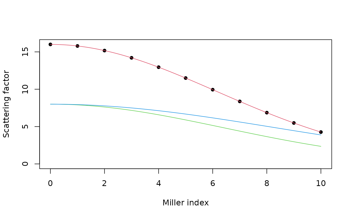
plot(h,fval,pch=16,xlab="Miller index",ylab="Scattering factor",
     ylim=c(0,16))

# Continuous resolution
h <- seq(0,10,length=1000)
fval <- scafac(h,a,Zj,occj,Bj)
points(h,fval,type="l",col=2)

# Scattering curve for a lighter atom
Zj <- 8
fval <- scafac(h,a,Zj,occj,Bj)
points(h,fval,type="l",col=3)

# Scattering curve for the same atom, just with smaller Bj (colder)
Bj <- 10
fval <- scafac(h,a,Zj,occj,Bj)
points(h,fval,type="l",col=4)